Spatiotemporal Patterns Formed by a Discrete Nutrient-Phytoplankton Model with Time Delay

Zhang, Feifan; Zhou, Wenjiao; Yao, Lei; Wu, Xuanwen; Zhang, Huayong

doi:https://doi.org/10.1155/2020/8541432

Complexity

On this page

Abstract Introduction Model and Analysis Discussion and Conclusions Appendix Data Availability Conflicts of Interest Acknowledgments References Copyright Related Articles

Research Article | Open Access

Volume 2020 | Article ID 8541432 | https://doi.org/10.1155/2020/8541432

Spatiotemporal Patterns Formed by a Discrete Nutrient-Phytoplankton Model with Time Delay

Feifan Zhang,¹Wenjiao Zhou,¹Lei Yao,¹Xuanwen Wu,¹and Huayong Zhang¹

Academic Editor: Eric Campos-Canton

Received20 Sept 2019

Revised27 Nov 2019

Accepted11 Dec 2019

Published09 Jan 2020

Abstract

In this research, a continuous nutrient-phytoplankton model with time delay and Michaelis–Menten functional response is discretized to a spatiotemporal discrete model. Around the homogeneous steady state of the discrete model, Neimark–Sacker bifurcation and Turing bifurcation analysis are investigated. Based on the bifurcation analysis, numerical simulations are carried out on the formation of spatiotemporal patterns. Simulation results show that the diffusion of phytoplankton and nutrients can induce the formation of Turing-like patterns, while time delay can also induce the formation of cloud-like pattern by Neimark–Sacker bifurcation. Compared with the results generated by the continuous model, more types of patterns are obtained and are compared with real observed patterns.

1. Introduction

Phytoplankton is the main producer of aquatic ecosystems and forms the basis of food webs [1]. The growth of phytoplankton can determine the behavioral space of plankton directly and then even affects the development of the whole aquatic ecosystem. As the spatial and temporal distribution/self-organization of phytoplankton is quite visible, it can reflect the “structure” of the aquatic ecosystem, which also reveals the strategy that phytoplankton takes to adapt to environmental changes. Therefore, investigation on the self-organization of phytoplankton has been essential to the understanding of ecosystem evolution and remains a hot topic in ecosystem dynamics and complexity.

One of the most striking manifestations of biological ocean dynamics is the proliferation of particularly dense phytoplankton, which often forms marvelous patterns with unexpectedly clear boundaries, such as banded patterns, chaotic patterns, and solitons. [2–4]. These patterns are usually produced by the interaction between the behavior of organisms (sinking, floating, or swimming) and the surrounding physical flow [3]. By examining the structure of dense phytoplankton mass reproduction, the local physical dynamics of living organisms, as well as behavioral and physiological responses, can be obtained. Patterns of some accumulations are the reflection of specific flows; observation of these visible patterns may reveal underlying dynamics [3]. However, the formation mechanism of these patterns is still unclear, and further research is urgently needed.

Since the environmental factors in the phytoplankton ecosystem vary with time, simple statistical models cannot accurately describe the dynamic process of phytoplankton growth in time and space. Therefore, the establishment of a dynamic model of plankton populations is an important method to study the physical and biological processes of plankton [5–10]. In 1949, Riley et al. established a vertical one-dimensional ecological dynamics model to simulate the seasonal changes of plankton in the North Sea of Europe, which symbolizes the study of aquatic ecosystems from qualitative description to the era of quantitative simulation [11]. In the same year, Monod, the founder of modern cell growth, proposed the famous Monod kinetic model, which describes the effect of substrate concentration on the cell growth rate, laying the foundation for the development of cell growth dynamics, thus promoting the development of phytoplankton growth dynamics [12]. After the Monod model was proposed, it was widely used in the study of phytoplankton growth dynamics [13–19] and found that the Monod model is very suitable under certain conditions. Ye et al. used the Monod model to quantitatively study the relationship between phytoplankton biomass and nutrients in Taihu Lake [20]. It was found that total nitrogen is a key factor affecting the growth of phytoplankton, and eutrophication of lakes to phytoplankton growth has served as positive feedback. However, some studies have shown that the relationship between phytoplankton growth and nutrients does not follow the Monod model, which means that the Monod model has limitations [21]. Dugdale used the Michaelis–Menten model to describe the absorption of nutrients by planktonic algae under steady-state conditions [22, 23], revealing the effects of limited nutrient salts on the growth of planktonic algae. Studies have shown that it is feasible to describe the quantitative relationship between phytoplankton growth rate and nutrient salt concentration with Michaelis–Menten model under steady-state conditions [24].

Reaction-diffusion equations have been widely used to describe temporal and spatial complexity in ecology [25–33]. Time delay always exists and plays an important role in dynamical systems, and some dynamical phenomena could be affected by the time delay [34–37]. Turing bifurcation helps with the explanation of self-organization. Usually, Turing analysis is carried out on the basis of continuous models. In ecosystems, discrete models can generate more dynamical behaviors, which undoubtedly reflect ecological complexity [38, 39]. It is worth noting that numerical simulation is actually based on discrete forms of continuous systems, which automatically give numerical simulation algorithms. Therefore, the discrete form is the natural link between the actual model and the simulation. At the same time, in many cases, the environment exhibits considerable spatial variability and is best considered using spatial discrete methods [40–43]. Wang et al. studying the discrete forms of the Gierer–Meinhardt system found that discrete systems lead to more complex nonlinear behaviors and new dynamic phenomena than continuous forms. In addition, for the discrete time and space G-M system, they found a new instability mechanism, pronunciation flip-Turing instability [44]. In addition, when we apply Turing analysis on discrete models, there are some differences. First, the solution space of the continuous Turing model is infinite dimension, while the corresponding discretization model is in finite dimension. Secondly, in the linearization analysis of Turing bifurcation, elliptic operators have infinite eigenvalues and eigenvalue sequences are unbounded, while discrete elliptic operators have only finite eigenvalues. Therefore, it is of great significance to further reveal the formation mechanism of space-time self-organization by discretizing the reaction-diffusion equation in space and time. In this research, we use the N-S bifurcation theorem described by Guckenheimer and Holmes [45] to determine the conditions under which bifurcation occurs.

Therefore, in this research, we will investigate the self-organization of phytoplankton in a spatiotemporal discrete nutrient-phytoplankton model with time delay. The model is obtained through the discretization of a continuous nutrient-phytoplankton model proposed by Dai et al. [46]. Based on the discrete model, Neimark–Sacker bifurcation analysis and Turing bifurcation analysis are carried out, and parameter space is obtained correspondingly. Numerical simulations are then carried out using MATLAB (2011a) on the formation of phytoplankton patterns with different parameter values. Considering the pattern types and holistic shapes, the simulated phytoplankton patterns are compared with those observed in the real world. In addition, we also illustrate the results that can be obtained by the discrete model in the research are far more than those by the continuous model in [46].

2. Model and Analysis

2.1. A Discrete Spatiotemporal Nutrient-Phytoplankton Model with Delay

Considering the rate of diffusion of nutrients and phytoplankton is different in real-world systems, therefore, in this paper, we obtain the following spatial nutrient-phytoplankton models based on Ref. [46]:where and represent nutrient concentration and the population biomass of phytoplankton, respectively. All parameters are non-negative and . Let and .

In the Turing instability analysis, people often give theoretical analysis to the continuous model, while the Turing pattern simulation undoubtedly adopts the corresponding discretization model. It is important to discretize the reaction-diffusion equation in space-time, which is of great significance for further revealing the formation mechanism of space-time self-organized structure. Therefore, in this paper, we consider the model on a lattice, and the two variables can be expressed as and ( and ), which represent the nutrient concentration and the phytoplankton density in lattice at time , respectively. According to the former research works of [39, 47], there are two stages, reaction stage and diffusion stage, when we discretize the continuous model (equation (1)). Meanwhile, we use a standard second-order central finite difference scheme to discretize (1) in space. The spatial dispersal stage, that is, diffusion, is considered firstly aswhere , , , and are the time interval and space interval. denotes the discrete form of the Laplacian operator:

Then, we consider the reaction stage:

Boundary conditions are set as periodic conditions as follows:

Equations (2) and (4) including both diffusion and reaction stages are defined as our discrete model. According to the spatial homogeneity of the discrete system, with all , and , we have

From (6), together with (2)–(4), then the homogeneous dynamics satisfies the following equation:where , we rewrite equation (7) into the form of maps:

In the sequel, we use (8) to analyze the homogeneous dynamics of equations (2)–(4).

2.2. Analysis of the Stability of the Homogeneous Steady State

The fixed point of map (8) is a homogeneous steady state of equations (2)–(4). So, we carry out the analysis of the stability about the fixed point of map (8). When both the delay and the diffusion are not considered, it is easy to see that map (8) has two fixed points: and , where and . The sufficient and necessary conditions for that is positive are as follows:

The Jacobian matrix method is used to determine the local stability of fixed points. Since pattern formation requires the nontrivial homogeneous stationary state, which is corresponding to the fixed point , we just concern the stability of . The corresponding Jacobian is given by

The two eigenvalues of matrix (10) are as follows:where

According to the criterion of stability of the fixed point, if and , the fixed point is locally asymptotically stable. As shown in the previous research [48], this criterion of stability is equivalent to . Through calculations, the conditions for to be locally asymptotically stable are determined as follows:where

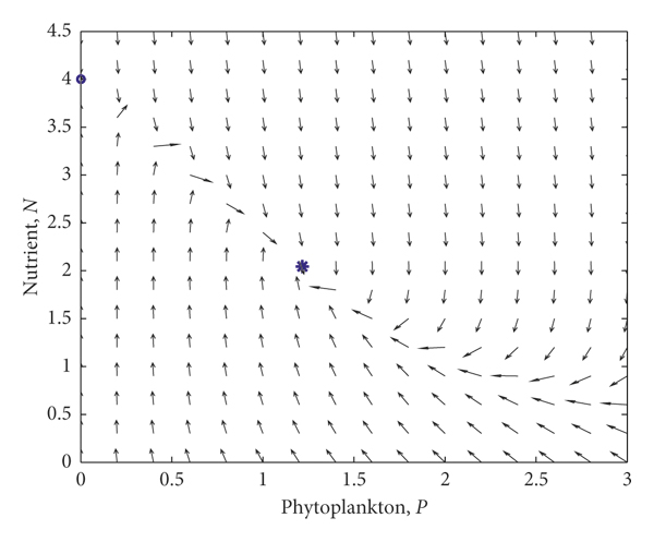
The dynamics of the discrete model without spatial diffusions can be shown in Figure 1, and the following bifurcations and simulations are all carried out in this situation. Note that, in the discrete system, the arrows in the figure represent the direction of iteration rather than dynamic flow. And is considered, as when time delay increases, the following bifurcation will occur.

2.3. Bifurcation Analysis of the Homogeneous Steady State

2.3.1. Neimark–Sacker Bifurcation Analysis

In this part, we consider Neimark–Sacker bifurcation of equations (2)–(4) when is small. We first make a corresponding change to equation (1) and obtain equation (17) and then discretize equation (17) to obtain map (18).

If is small, , put it into equation (1) and obtainin which

Taylor expansion of at without considering the higher order nonlinear part and equation (1) can be written aswhere and . Therefore, equation (8) can be expressed as the following map:

According to [48], the first condition of Neimark–Sacker bifurcation requires the eigenvalues at a fixed point, and are conjugate and their modules are 1, shown asin which have been shown in Appendix A.

Then, we can get

By calculation, we can obtain the Neimark–Sacker bifurcation point :

Under the satisfaction of conditions (22) and (23), the fixed point of map (18) is translated to the origin by the following translation:

Then, map (18) is transformed intowhere have been shown in Appendix A with .

The second condition for Neimark–Sacker bifurcation requiresin whichwhere and are described in equation (21) with . Then, we can obtain

On the basis of map (25), the canonical form is studied to obtain the last condition for the occurrence of Neimark–Sacker bifurcation. The invertible transformation is applied:

To map (25), then the map becomeswhere

The second-order and third-order partial derivatives of and at are calculated as

The third condition of Neimark–Sacker bifurcation requiresin which

After calculation, the third condition for Neimark–Sacker can be expressed asin which

Based on the above calculations, when the conditions (23), (28), and (35) are satisfied, Neimark–Sacker bifurcation occurs at the fixed point . Moreover, when and , then an attracting invariant closed curve bifurcates from the fixed point for ; otherwise, when and , a repelling invariant closed curve bifurcates from the fixed point for .

In Figure 2(a), the parameter space of time delay and input rate is shown. Zone I represents that when the input rate of nutrient is low, positive fixed point does not exist. Zone II and III represent no bifurcation and bifurcation area around the fixed point . And Figure 2(b) shows the bifurcation diagram when and . The Hopf bifurcation point is not suitable here with a time step not small enough, while the calculated Neimark–Sacker bifurcation point is more correct compared with the simulated bifurcation point. This difference can be shown in Figure 2(d): cannot be equal to 0.2, but in the discrete model, when , Neimark–Sacker bifurcation occurs and drives the system from stable fixed point to quasiperiodic dynamics. When time delay satisfy both and , the dynamics of the continuous model (with as in [46]) and the discrete model () show differences: Hopf bifurcation induces the continuous system into a limit cycle (Figure 2(c)); Neimark–Sacker bifurcation induces the discrete system into quasiperiodic iteration and the amplitude of variables is larger.

(a)

(b)

(c)

(d)

(e)

2.3.2. Turing Bifurcation Analysis

In this part, we consider Turing bifurcation of equations (2)–(4) when . Turing bifurcation requires two conditions. Firstly, a nontrivial homogeneous stationary state exists and is stable to spatially homogeneous perturbations, which has been obtained in the above section. Secondly, the stable stationary state is unstable to at least one type of spatially heterogeneous perturbations. This paper is based on the method of Bai and Zhang to do Turing bifurcation analysis of the discrete model [49]. We first consider the following eigenvalue equation:with periodic boundary conditions:

When and , we set , put it into equation (38), and obtain . Then, we can get

Substituting into equation (37), we obtain that

By calculating , then, using equation (39) we can get

Turing bifurcation is caused by the lack of spatial symmetry. To analyze the Turing bifurcation, a spatially nonuniform perturbation is applied at the spatially uniform state . The equation for spatially nonuniform perturbations can be expressed as

Noticing and , and the values of the two cannot be constant to 0. Substituting equation (42) into equations (2)–(4) leads to the following equation:

The high-order terms in the above equations can be ignored when the disturbance is very weak. Using the corresponding characteristic function of the eigenvalue to multiply equation (43), we obtain

Summing equation (44) for all and gives the following equation:

Let and , combined boundary conditions (38), equation (45) can be transformed into the following form:

At this time, we know that a progressive solution of equations (2)–(4) with boundary conditions (5) is . Therefore, we know that if the solution of the equation (46) is unstable, it will cause the equations (2)–(4) to be unstable. The eigenvalues of equations (2)–(4) are as follows:in which

Here, , , , and are denoted for reminding that they are dependent on . Based on the two eigenvalues, we define

The occurrence of Turing bifurcation needs to satisfy . According to this condition, we can determine the critical value of Turing bifurcation occurring, which can be described as follows:(1)If is satisfied in a small neighborhood of , the critical value satisfies (2)If is satisfied in a small neighborhood of , the critical value satisfies

and determine the critical conditions for the occurrence of Turing bifurcation in discrete systems. From this critical condition, the conditions for the formation of the Turing pattern can be obtained. By simplifying the two cases described above, it can be known that Turing instability occurs and leads to the formation of spatial heterogeneity patterns when .

Then, we discuss the influence of the diffusion coefficients and on the model. We use the following parameter values: , , , , , , , , , , , , and . The discrete model is solved numerically in a rectangular spatial grid consisting of 100 × 100 units, and periodic boundary conditions are adopted. As shown in Figure 3, Turing bifurcation can be displayed via the change of eigenvalue . In Figure 3(a), we can see that the perturbation parameters and have symmetrical effects on the eigenvalues. Therefore, for convenience of observation, let , then we can get the change in the eigenvalue to , as shown in Figure 3(b). If there is no disturbance, the system will be at a stable point. But, when there is disturbance, Turing bifurcation can happen. According to Figure 3(b), we can know that if the diffusion coefficient , then the eigenvalue of the system will not make the eigenvalue greater than 1 with the increase of the perturbation parameter; at this time, Turing bifurcation will not occur. When , the curve is tangent to the straight line , that is, only if the diffusion coefficient , the value of the eigenvalue will exceed 1 as the disturbance coefficient increases; at this time, Turing bifurcation will occur in the system.

(a)

(b)

3. Numerical Simulations

In this section, numerical simulations on the formation of phytoplankton are carried out focusing on three aspects including time delay and diffusion coefficients and . Note that initial conditions are set as homogeneous steady states on 100 × 100 (mostly) lattice with ±5% random perturbations. Then simulated patterns are compared with real observed patterns.

3.1. Effects of Time Delay on the Pattern Formation

According to the stability analysis and Neimark–Sacker bifurcation analysis, time delay can cause the instability of the system. As shown in Figure 4, with given parameter values, the critical value of can be calculated as . Thus, we take , , and and obtain Figures 4(a)–4(c) respectively. Figures 4(a) and 4(b) show that when , there is no spatial patterns. Figure 4(c) clearly shows the formation of a Neimark–Sacker type pattern when . From the simulated patterns, we can see that simulations are consistent with the Neimark–Sacker analysis.

(a)

(b)

(c)

Figure 5 shows a time series of phytoplankton pattern formation process from initial conditions to self-organization when . Small patches can be formed at the beginning (Figures 5(b) and 5(c)), and then gradually forming spirals (Figure 5(d)). The spirals will break with time, and reform afterwards (Figures 5(e)–5(g)). Then cloud-like patterns will finally be formed (Figures 5(h) and 5(i)).

(a)

(b)

(c)

(d)

(e)

(f)

(g)

(h)

(i)

3.2. Effects of Diffusion Coefficients on the Pattern Formation

Based on the Turing bifurcation analysis in Section 2.3.2, we can see that the diffusion coefficient can induce the occurrence of Turing bifurcations, and the critical value is . Figure 6(a) shows that there is no pattern, while in Figure 6(b) we can clearly see the appearance of a typical banded Turing-type pattern. In addition, diffusion coefficient can also induce the occurrence of Turing bifurcation as shown in Figure 6(c). The simulations are quite consistent with the above analysis of Turing bifurcation.

(a)

(b)

(c)

In order to show the formation process of Turing-type patterns, two sets of values are selected: , and , . Figure 7 shows that, at the beginning, random distribution of phytoplankton starts to form a labyrinth pattern (Figures 7(b)–7(d)), and then some patches die out and form some thin stripes (Figures 7(f) and 7(g)). Finally, the number of stripes decreases over time (Figures 7(h) and 7(i)). Figure 8 shows a similar process of pattern formation with slight differences.

(a)

(b)

(c)

(d)

(e)

(f)

(g)

(h)

(i)

(a)

(b)

(c)

(d)

(e)

(f)

(g)

(h)

(i)

Note that when time delay satisfies the Neimark-Sacker bifurcation condition and coefficients and satisfy Turing bifurcation condition, simulations on pattern formation will be different. As shown in Figure 9, the general process of pattern formation is similar to that when time delay (see Figure 7). Note that as shown in Figure 9(d) with , the same formation stage of patterns can be obtained in Figure 7(e) with . This reveals that the time delay will not change the pattern type in this situation, but will cause the delay of pattern formation stages, which is reasonable and consistent with the research of [46].

(a)

(b)

(c)

(d)

(e)

(f)

(g)

(h)

(i)

3.3. Comparison between Simulated Patterns and Real Observed Patterns

From numerical simulations, mainly two types of patterns are obtained: cloud-like patterns (Figure 10(a)) and banded patterns (Figures 11(a), 11(c), and 11(e)). Some observed patterns of phytoplankton are found and can be briefly compared with the simulated patterns from the holistic shapes. Figure 10(b) is the blooming phenomenon in the Barents Sea and shows similarity to the simulated cloud pattern (Figure 10(a)).

(a)

(b)

(a)

(b)

(c)

(d)

(e)

(f)

Figures 11(b) and 11(f) are phytoplankton bloom images taken in the waters near Shenzhen, China, in 2014, and Figure 11(d) is a large area phytoplankton bloom image of Noctiluca scintillans taken in the waters near Rizhao in Shandong, China in 2012. The simulated banded patterns are similar to the observed patterns. But note that we can only compare the holistic shapes or types of the patterns due to the unknown of real pattern scales, and further research should be done to explore more detailed comparison on spatial scales of the patterns.

4. Discussion and Conclusions

Through theoretical analysis and numerical simulation, the principle of space-time dynamics of phytoplankton growth and the formation process of spatial pattern distribution of phytoplankton population are explored. We mainly study the effects of time delay and, diffusion coefficients on the spatiotemporal dynamics of phytoplankton growth. The conclusions of theoretical studies and the results of numerical simulations can show that: (1) time delay does not affect the stability of the stable fixed point , but the time delay may affect the whole process; (2) when time delay exists and is greater than a certain critical value , the time delay can not only lead to the instability of the stable fixed point , but also form a cloud Neimark–Sacker pattern through Neimark–Sacker instability; (3) when , by changing the value of or to make all the eigenvalues of the diffusion term are greater than 1, then Turing bifurcation occurs. A band-shaped Turing pattern can be formed.

Both the continuous model (original model in [46]) and the discrete model in this research are reaction-diffusion models, and they have the same functional responses. The differences between the two models are as follows: in the continuous model, reaction process and diffusion process occurs at the same time, while in the discrete model, the occurring order of reaction process and diffusion process can be varied, to be exactly in this research, diffusion process occur first and then reaction process. The main reason for us to calculate the diffusion process first is that spatial movements are quicker than reaction in the nutrient-phytoplankton system in the real world.

From the simulated patterns in this research, we can see that more complex and more types of patterns can be obtained with the discrete model than the continuous model. For example, Figure 10(a) is the simulated pattern with a similar type to the only simulated pattern in [46]. Besides, spotted, banded, and some mixed patterns are obtained in this research. This is reasonable, as Dai et al. [46] only did the Turing bifurcation. However, even with the same bifurcations, discrete models can still generate more complex patterns, due to the flexible of both time and space steps. Although continuous PDEs are still the main type of model that are used in pattern formation, many research studies on discrete dynamic systems have shown that spatiotemporal discrete models are not only more related to realistic processes but also can generate more complex dynamics [38, 39, 43, 44]. And more work could be done to explore the bifurcations induced by time step variation.

Appendix

A. Symbols Not Explained in Section 2

Data Availability

Codes related to the simulations can be made available on request (china907a@163.com).

Conflicts of Interest

The authors declare that they have no conflicts of interest.

Acknowledgments

The authors would like to acknowledge with great gratitude for the supports of the Major Science and Technology Program for Water Pollution Control and Treatment (no. 2017ZX07101002) and the National Natural Science Foundation of China (Grant nos. 11875126 and 11771140).

References

D. M. Anderson, “Turning back the harmful red tide,” Nature, vol. 388, no. 6642, pp. 513-514, 1997.
View at: Publisher Site | Google Scholar
Y.-H. Ahn, P. Shanmugam, J.-H. Ryu, and J.-C. Jeong, “Satellite detection of harmful algal bloom occurrences in Korean waters,” Harmful Algae, vol. 5, no. 2, pp. 213–231, 2006.
View at: Publisher Site | Google Scholar
P. J. S. Franks, “Spatial patterns in dense algal blooms,” Limnology and Oceanography, vol. 42, no. 5, pp. 1297–1305, 1997.
View at: Publisher Site | Google Scholar
W. Q. Chen, Q. F. Guan, C. F. Jiang, F. F. Zhang, and L. Wang, “Nonautonomous motion study on accelerated and decelerated lump waves for a (3 + 1)-dimensional generalized shallow water wave equation with variable coefficients,” Complexity, vol. 2019, Article ID 6287461, 8 pages, 2019.
View at: Publisher Site | Google Scholar
A. Huppert, B. Blasius, R. Olinky, and L. Stone, “A model for seasonal phytoplankton blooms,” Journal of Theoretical Biology, vol. 236, no. 3, pp. 276–290, 2005.
View at: Publisher Site | Google Scholar
M. Rehim and M. Imran, “Dynamical analysis of a delay model of phytoplankton-zooplankton interaction,” Applied Mathematical Modelling, vol. 36, no. 2, pp. 638–647, 2012.
View at: Publisher Site | Google Scholar
A. Sharma, A. K. Sharma, and K. Agnihotri, “The dynamic of plankton-nutrient interaction with delay,” Applied Mathematics and Computation, vol. 231, pp. 503–515, 2014.
View at: Publisher Site | Google Scholar
G.-Q. Sun, “Mathematical modeling of population dynamics with Allee effect,” Nonlinear Dynamics, vol. 85, no. 1, pp. 1–12, 2016.
View at: Publisher Site | Google Scholar
X. Yu, S. Yuan, and T. Zhang, “The effects of toxin-producing phytoplankton and environmental fluctuations on the planktonic blooms,” Nonlinear Dynamics, vol. 91, no. 3, pp. 1653–1668, 2017.
View at: Publisher Site | Google Scholar
F. Zhang, H. Zhang, M. R. Evans, and T. Huang, “Vegetation patterns generated by a wind driven sand-vegetation system in arid and semi-arid areas,” Ecological Complexity, vol. 31, pp. 21–33, 2017.
View at: Publisher Site | Google Scholar
G. A. Riley, H. Stommel, and D. F. Bumpus, “Quantitative ecology of plankton of Western North Atlantic,” Bulletin of the Bingham Oceanographic Collection, vol. 169, pp. 1–12, 1949.
View at: Google Scholar
J. Monod, “The growth of bacterial cultures,” Annual Review of Microbiology, vol. 3, no. 1, pp. 371–394, 1949.
View at: Publisher Site | Google Scholar
S. Babel and S. Takizawa, “Microfiltration membrane fouling and cake behavior during algal filtration,” Desalination, vol. 261, no. 1-2, pp. 46–51, 2010.
View at: Publisher Site | Google Scholar
X. Bai, P. Lant, and S. Pratt, “The contribution of bacteria to algal growth by carbon cycling,” Biotechnology and Bioengineering, vol. 112, no. 4, pp. 688–695, 2015.
View at: Publisher Site | Google Scholar
J. Caperon, “Population growth response of isochrysis galbana to nitrate variation at limiting concentrations,” Ecology, vol. 49, no. 5, pp. 866–872, 1968.
View at: Publisher Site | Google Scholar
J. C. Goldman and E. J. Carpenter, “A kinetic approach to the effect of temperature on algal growth,” Limnology and Oceanography, vol. 19, no. 5, pp. 756–766, 1974.
View at: Publisher Site | Google Scholar
J. P. Grover, “Phosphorus-dependent growth kinetics of 11 species of freshwater algae,” Limnology and Oceanography, vol. 34, no. 2, pp. 341–348, 1989.
View at: Publisher Site | Google Scholar
J. P. Grover, “Resource competition in a variable environment: phytoplankton growing according to monod’s model,” The American Naturalist, vol. 136, no. 6, pp. 771–789, 1990.
View at: Publisher Site | Google Scholar
S. Park and Y. Li, “Integration of biological kinetics and computational fluid dynamics to model the growth of Nannochloropsis salinain an open channel raceway,” Biotechnology and Bioengineering, vol. 112, no. 5, pp. 923–933, 2015.
View at: Publisher Site | Google Scholar
C. Ye, Z. Shen, T. Zhang, M. Fan, Y. Lei, and J. Zhang, “Long-term joint effect of nutrients and temperature increase on algal growth in Lake Taihu, China,” Journal of Environmental Sciences, vol. 23, no. 2, pp. 222–227, 2011.
View at: Publisher Site | Google Scholar
E. A. Laws, S. Pei, and P. Bienfang, “Phosphate-limited growth of the marine diatom Thalassiosira weissflogii (Bacillariophyceae): evidence of non-monod growth kinetics,” Journal of Phycology, vol. 49, no. 2, pp. 241–247, 2013.
View at: Publisher Site | Google Scholar
R. C. Dugdale, “Nutrient limitation in the sea: dynamics, identification, and significance1,” Limnology and Oceanography, vol. 12, no. 4, pp. 685–695, 1967.
View at: Publisher Site | Google Scholar
L. Michaelis and M. L. Menten, “Die kinetik der invertin wirkung,” Biochemische Zeitschrift, vol. 49, pp. 334–336, 1913.
View at: Google Scholar
M. Latasa and E. Berdalet, “Effect of nitrogen or phosphorus starvation on pigment composition of cultured Heterocapsa sp,” Journal of Plankton Research, vol. 16, no. 1, pp. 83–94, 1994.
View at: Publisher Site | Google Scholar
J. Arrieta, A. Barreira, and I. Tuval, “Microscale patches of nonmotile phytoplankton,” Physical Review Letters, vol. 114, no. 12, Article ID 128102, 2015.
View at: Publisher Site | Google Scholar
K. Chakraborty and V. Manthena, “Modelling and analysis of spatio-temporal dynamics of a marine ecosystem,” Nonlinear Dynamics, vol. 81, no. 4, pp. 1895–1906, 2015.
View at: Publisher Site | Google Scholar
S. Ghorai and S. Poria, “Turing patterns induced by cross-diffusion in a predator-prey system in presence of habitat complexity,” Chaos, Solitons & Fractals, vol. 91, pp. 421–429, 2016.
View at: Publisher Site | Google Scholar
S. Ghorai and S. Poria, “Pattern formation in a system involving prey–predation, competition and commensalism,” Nonlinear Dynamics, vol. 89, no. 2, pp. 1309–1326, 2017.
View at: Publisher Site | Google Scholar
L. Li, Z. Jin, and J. Li, “Periodic solutions in a herbivore-plant system with time delay and spatial diffusion,” Applied Mathematical Modelling, vol. 40, no. 7-8, pp. 4765–4777, 2016.
View at: Publisher Site | Google Scholar
G. Q. Sun, C. H. Wang, L. L. Chang, Y.-P. Wu, L. Li, and Z. Jin, “Effects of feedback regulation on vegetation patterns in semi-arid environments,” Applied Mathematical Modelling, no. 61, pp. 200–215, 2018.
View at: Publisher Site | Google Scholar
R. Yang, “Bifurcation analysis of a diffusive predator-prey system with Crowley-Martin functional response and delay,” Chaos, Solitons & Fractals, vol. 95, pp. 131–139, 2017.
View at: Publisher Site | Google Scholar
F. Zhang, H. Zhang, T. Huang, T. Meng, and S. Ma, “Coupled effects of turing and neimark-sacker bifurcations on vegetation pattern self-organization in a discrete vegetation-sand model,” Entropy, vol. 19, no. 9, p. 478, 2017.
View at: Publisher Site | Google Scholar
X. Zhang and H. Zhao, “Dynamics and pattern formation of a diffusive predator–prey model in the presence of toxicity,” Nonlinear Dynamics, vol. 95, no. 3, pp. 2163–2179, 2018.
View at: Publisher Site | Google Scholar
P. Mishra, S. N. Raw, and B. Tiwari, “Study of a Leslie-Gower predator-prey model with prey defense and mutual interference of predators,” Chaos, Solitons & Fractals, vol. 120, pp. 1–16, 2019.
View at: Publisher Site | Google Scholar
A. Otto, J. Wang, and R. Günter, “Delay-induced wave instabilities in single-species reaction-diffusion systems,” Physical Review E, vol. 96, no. 5, Article ID 052202, 2017.
View at: Publisher Site | Google Scholar
F. A. Rihan, C. Tunc, S. H. Saker, S. Lakshmanan, and R. Rakkiyappan, “Applications of delay differential equations in biological systems,” Complexity, vol. 2018, Article ID 4584389, 3 pages, 2018.
View at: Publisher Site | Google Scholar
Z. Zhang, R. K. Upadhyay, R. Agrawal, and J. Datta, “The gestation delay: a factor causing complex dynamics in gause-type competition models,” Complexity, vol. 2018, Article ID 1589310, 21 pages, 2018.
View at: Publisher Site | Google Scholar
T. Huang and H. Zhang, “Bifurcation, chaos and pattern formation in a space- and time-discrete predator-prey system,” Chaos, Solitons & Fractals, vol. 91, pp. 92–107, 2016.
View at: Publisher Site | Google Scholar
D. C. Mistro, L. A. Díaz Rodrigues, and S. Petrovskii, “Spatiotemporal complexity of biological invasion in a space- and time-discrete predator–prey system with the strong Allee effect,” Ecological Complexity, vol. 9, pp. 16–32, 2012.
View at: Publisher Site | Google Scholar
H. N. Comins, M. P. Hassell, and R. M. May, “The spatial dynamics of host—parasitoid systems,” The Journal of Animal Ecology, vol. 61, no. 3, pp. 735–748, 1992.
View at: Publisher Site | Google Scholar
X. Liu and D. Xiao, “Complex dynamic behaviors of a discrete-time predator-prey system,” Chaos, Solitons & Fractals, vol. 32, no. 1, pp. 80–94, 2007.
View at: Publisher Site | Google Scholar
S. M. White and K. A. J. White, “Relating coupled map lattices to integro-difference equations: dispersal-driven instabilities in coupled map lattices,” Journal of Theoretical Biology, vol. 235, no. 4, pp. 463–475, 2005.
View at: Publisher Site | Google Scholar
F. Zhang, H. Zhang, S. Ma, T. Meng, T. Huang, and H. Yang, “Self-organized patterns induced by neimark-sacker, flip and turing bifurcations in a discrete predator-prey model with lesie-gower functional response,” Entropy, vol. 19, no. 6, p. 258, 2017.
View at: Publisher Site | Google Scholar
J. Wang, Y. Li, S. Zhong, and X. Hou, “Analysis of bifurcation, chaos and pattern formation in a discrete time and space Gierer Meinhardt system,” Chaos, Solitons & Fractals, vol. 118, pp. 1–17, 2019.
View at: Publisher Site | Google Scholar
J. Guckenheimer and P. Holmes, Nonlinear Oscillations, Dynamical Systems, and Bifurcations of Vector Fields, Springer Science & Business Media, Berlin, Germany, 2013.
C. J. Dai, M. Zhao, and H. G. Yu, “Dynamics induced by delay in a nutrient–phytoplankton model with diffusion,” Ecological Complexity, vol. 26, pp. 29–36, 2016.
View at: Publisher Site | Google Scholar
D. Punithan, D.-K. Kim, and R. Mckay, “Spatio-temporal dynamics and quantification of daisyworld in two-dimensional coupled map lattices,” Ecological Complexity, vol. 12, pp. 43–57, 2012.
View at: Publisher Site | Google Scholar
T. Huang, H. Zhang, H. Yang, N. Wang, and F. Zhang, “Complex patterns in a space-and time-discrete predator-prey model with Beddington-DeAngelis functional response,” Communications in Nonlinear Science and Numerical Simulation, vol. 43, pp. 182–199, 2017.
View at: Publisher Site | Google Scholar
L. Bai and G. Zhang, “Nontrivial solutions for a nonlinear discrete elliptic equation with periodic boundary conditions,” Applied Mathematics and Computation, vol. 210, no. 2, pp. 321–333, 2009.
View at: Publisher Site | Google Scholar

Copyright

Copyright © 2020 Feifan Zhang et al. This is an open access article distributed under the Creative Commons Attribution License, which permits unrestricted use, distribution, and reproduction in any medium, provided the original work is properly cited.

PDF Download Citation

Download other formats

Order printed copies

Views

470

Downloads

839

Citations